
EEG Wave Detection and Analysis#
Project: EEG Slow Wave Detection and Analysis#
- This project was published in the following paper:
- Carvalho DZ, Kremen V, Mivalt F, St Louis EK, McCarter SJ, Bukartyk J, Przybelski SA, Kamykowski MG, Spychalla AJ, Machulda MM, Boeve BF, Petersen RC, Jack CR Jr, Lowe VJ, Graff-Radford J, Worrell GA, Somers VK, Varga AW, Vemuri P. Non-rapid eye movement sleep slow-wave activity features are associated with amyloid accumulation in older adults with obstructive sleep apnoea. Brain Commun. 2024 Oct 7;6(5):fcae354. doi: 10.1093/braincomms/fcae354. PMID: 39429245; PMCID: PMC11487750.
Here we conveniently provide a standalone fully functional code example for analysis related to this project - One file example. This enables trialing this code without installing the whole Best Toolbox library. The codes were also embedded into the brainmaze_eeg Toolbox so they can be freely available upon installing the whole Brainmaze EEG Library. The documentation to the toolbox is available at Brainmaze EEG Documentation.
TBD TBD !!!! For more information on this specific project, see the page describing Wave Detection.
Acknowledgement#
F. Mivalt et V. Kremen et al., “Electrical brain stimulation and continuous behavioral state tracking in ambulatory humans,” J. Neural Eng., vol. 19, no. 1, p. 016019, Feb. 2022, doi: 10.1088/1741-2552/ac4bfd.F. Mivalt et V. Sladky et al., “Automated sleep classification with chronic neural implants in freely behaving canines,” J. Neural Eng., vol. 20, no. 4, p. 046025, Aug. 2023, doi: 10.1088/1741-2552/aced21.Gerla, V., Kremen, V., Macas, M., Dudysova, D., Mladek, A., Sos, P., & Lhotska, L. (2019). Iterative expert-in-the-loop classification of sleep PSG recordings using a hierarchical clustering. Journal of Neuroscience Methods, 317(February), 61?70. https://doi.org/10.1016/j.jneumeth.2019.01.013Kremen, V., Brinkmann, B. H., Van Gompel, J. J., Stead, S. (Matt) M., St Louis, E. K., & Worrell, G. A. (2018). Automated Unsupervised Behavioral State Classification using Intracranial Electrophysiology. Journal of Neural Engineering. https://doi.org/10.1088/1741-2552/aae5ab
Version#
Version 1.0 (2024-06-01) by V. Kremen (Kremen.Vaclav@mayo.edu)
Examples#
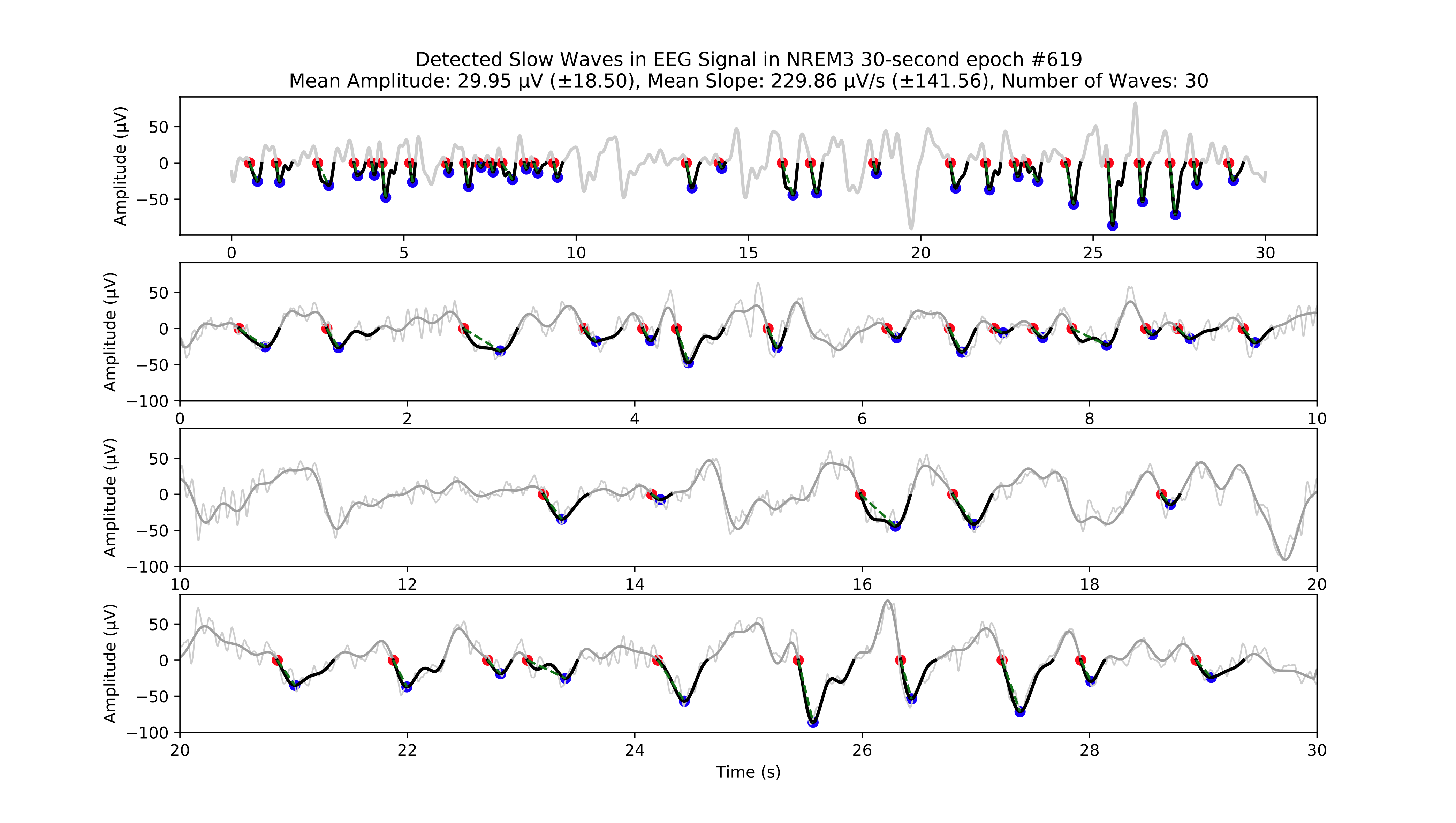
Example of individual slow wave detections.
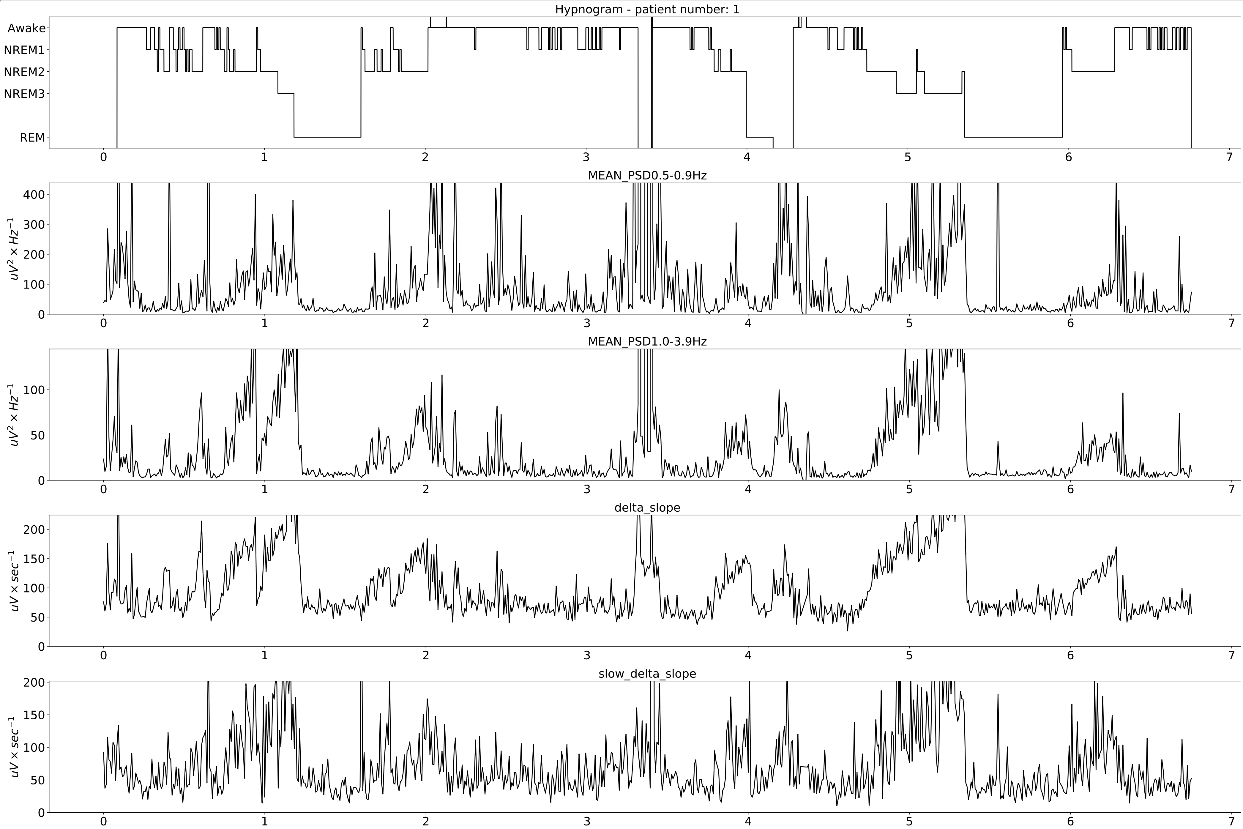
Extracted features for the whole night.
Code#
The code is also attached for convenience in here:
# region Description and Acknowledgements
#
# Code for extracting and analyzing electrophysiology features from EEG data and saving them to a CSV file.
# The program particularly analyzes one EEG signal from the Fz-(A1+A2)/2 channel and extracts features from it as a
# demonstration of the whole signal processing pipeline used in the project cited below.
#
# The code also plots the extracted features and saves the plots to PDF files including the PSD analysis figures.
# The code can also perform statistical analysis on the extracted features.
# The code can be run from the command line or from a Python IDE.
# The code requires the following packages to be installed: mne, pandas, numpy, scipy, plotly, tqdm, best, matplotlib.
# The code is written in Python 3.8.8. and calls also the SlowWaveDetect function from the SlowWaveDetector.py file.
# The code requires exported sleep saved in patient_one_data.pkl file placed in the directory of the script.
# The file contains EEG data for whole night recording with its sleep scoring
# and other metadata (such as sampling frequency).
#
# Acknowledgements:
# The code is part of the project of Analyzing EEG data from sleep studies for publication of manuscript:
# NREM sleep slow wave activity features are associated with amyloid accumulation in older adults with
# obstructive sleep apnea. By D. Carvalho et al., 2024
#
# The Feature Extractor uses the Behavioral State Analysis Toolbox (BEST) for feature extraction from raw EEG data.
# The BEST toolbox was developed during multiple projects we appreciate you acknowledge when using
# or inspired by this toolbox.
#
# Hyperlink to documentation of the BEST: https://best-toolbox.readthedocs.io/en/latest/index.html#
#
# Sleep classification and feature extraction
# F. Mivalt et V. Kremen et al., “Electrical brain stimulation and continuous behavioral state tracking in ambulatory humans,” J. Neural Eng., vol. 19, no. 1, p. 016019, Feb. 2022, doi: 10.1088/1741-2552/ac4bfd.
# F. Mivalt et V. Sladky et al., “Automated sleep classification with chronic neural implants in freely behaving canines,” J. Neural Eng., vol. 20, no. 4, p. 046025, Aug. 2023, doi: 10.1088/1741-2552/aced21.
# Gerla, V., Kremen, V., Macas, M., Dudysova, D., Mladek, A., Sos, P., & Lhotska, L. (2019). Iterative expert-in-the-loop classification of sleep PSG recordings using a hierarchical clustering. Journal of Neuroscience Methods, 317(February), 61?70. https://doi.org/10.1016/j.jneumeth.2019.01.013
# Kremen, V., Brinkmann, B. H., Van Gompel, J. J., Stead, S. (Matt) M., St Louis, E. K., & Worrell, G. A. (2018). Automated Unsupervised Behavioral State Classification using Intracranial Electrophysiology. Journal of Neural Engineering. https://doi.org/10.1088/1741-2552/aae5ab
# Kremen, V., Duque, J. J., Brinkmann, B. H., Berry, B. M., Kucewicz, M. T., Khadjevand, F., G.A. Worrell, G. A. (2017). Behavioral state classification in epileptic brain using intracranial electrophysiology. Journal of Neural Engineering, 14(2), 026001. https://doi.org/10.1088/1741-2552/aa5688
#
# The BEST was developed under projects supported by NIH Brain Initiative UH2&3 NS095495 Neurophysiologically-Based
# Brain State Tracking & Modulation in Focal Epilepsy, DARPA HR0011-20-2-0028 Manipulating and Optimizing Brain Rhythms
# for Enhancement of Sleep (Morpheus). Filip Mivalt was also partially supported by the grant FEKT-K-22-7649 realized
# within the project Quality Internal Grants of the Brno University of Technology (KInG BUT),
# Reg. No. CZ.02.2.69/0.0/0.0/19_073/0016948, which is financed from the OP RDE.
#
# License:
# This software is licensed under GNU license. For the details, see the LICENSE file in the root directory of this project.
# endregion Description and Acknowledgements
#
# Version 1.0 (2024-07-05) by V. Kremen (Kremen.Vaclav@mayo.edu)
# region Imports
import os
import warnings
import pandas as pd
import mne
import re
import math
from datetime import datetime
import concurrent.futures
from scipy.io import savemat, loadmat
import matplotlib.pyplot as plt
from scipy.signal import firwin, lfilter, freqz
import numpy as np
from scipy.signal import butter, firwin, filtfilt
from tqdm import tqdm
from best.files import get_files
from best.feature_extraction.SpectralFeatures import mean_frequency, median_frequency, mean_bands, relative_bands
from best.feature_extraction.FeatureExtractor import SleepSpectralFeatureExtractor
from SlowWaveDetector import SlowWaveDetect # Import the SlowWaveDetect function from SlowWaveDetector.py
from best.signal import buffer
from best import DELIMITER
# endregion imports
# region FILE_PATH
DATA_PATH = f'./patient_one_data.mat'
# endregion FILE_PATH
# region Parameters
ToPlotFigures = True # Do you want to print the figures? (True/False)
ToDoStats = False # Do you want to perform statistical analysis after you extracted features? (True/False)
features_path = 'Results_extraction.csv' # Where are going to be saved the extracted features?
features_to_plot = ['MEAN_PSD0.5-0.9Hz', 'MEAN_PSD1.0-3.9Hz', 'delta_slope', 'slow_delta_slope'] # Which features to plot?
plot_wave_images = True # Do you want to plot the wave images? (True/False)
# endregion parameters
# region Functions
def process_epoch(x_, x1_, x2_, t_, count, patient_id, hypnogram, fs_hypno, data_present, metadata, fsamp, path_edf):
epoch_result = {}
epoch_result['pt_id'] = patient_id
epoch_result['start'] = t_
epoch_result['end'] = t_ + 30
epoch_result['duration'] = 30
sleep_stage_in_epoch = math.ceil(hypnogram[int(((2 * t_ + 30) / 2) * fs_hypno)])
epoch_result['sleep_stage'] = sleep_stage_in_epoch
epoch_result['data_rate'] = (
np.sum(data_present[
int(t_ * fs_hypno) - 1:int(((t_ + 30) * fs_hypno)) - 1]) / (30 * fs_hypno))
total_record_time = metadata.loc[metadata['CLINIC'] == patient_id, 'TotalRecordTime'].values
if len(total_record_time) > 0 and t_ / 60 < total_record_time[0]:
epoch_result['phase'] = 0
elif len(total_record_time) > 0 and t_ / 60 > total_record_time[0]:
epoch_result['phase'] = 1
x__ = x_.copy()
x1__ = x1_.copy()
x2__ = x2_.copy()
warnings.filterwarnings('ignore', category=RuntimeWarning)
features, feature_names = FeatureExtractor(x_)
warnings.filterwarnings('default', category=RuntimeWarning)
epoch_result.update({name: feature for name, feature in zip(feature_names, np.concatenate(features))})
try:
sleep_stages = {
0: 'Awake',
1: 'NREM1',
2: 'NREM2',
3: 'NREM3',
5: 'REM',
9: 'UNKNOWN'
}
now = datetime.now()
date_time = now.strftime("%m-%d-%Y_%H-%M-%S")
nm = [pth for pth in path_edf.split('\\') if pth != '']
nm = nm[-1]
directory = f'Results\\{nm}'
file_name = f'{directory}\\{epoch}_EEG_extremes_{sleep_stages[sleep_stage_in_epoch]}_Delta_{date_time}.pdf'
results = SlowWaveDetect(x2__, fsamp, 0.5, 0.12, 5, file_name, sleep_stages[sleep_stage_in_epoch], epoch, False)
slow_waves, slow_wave_amplitudes, slow_wave_slopes, mean_amplitude, std_amplitude, mean_slope, std_slope, num_waves = results
if num_waves > 1:
epoch_result['delta_slope'] = mean_slope
epoch_result['delta_pk2pk'] = mean_amplitude
else:
epoch_result['delta_slope'] = np.nan
epoch_result['delta_pk2pk'] = np.nan
file_name = f'{directory}\\{epoch}_EEG_extremes_{sleep_stages[sleep_stage_in_epoch]}_SlowWave_{date_time}.pdf'
results = SlowWaveDetect(x1__, fsamp, 1, 0.55, 5, file_name, sleep_stages[sleep_stage_in_epoch], epoch, False)
slow_waves, slow_wave_amplitudes, slow_wave_slopes, mean_amplitude, std_amplitude, mean_slope, std_slope, num_waves = results
if num_waves > 2:
epoch_result['slow_delta_slope'] = mean_slope
epoch_result['slow_delta_pk2pk'] = mean_amplitude
else:
epoch_result['slow_delta_slope'] = np.nan
epoch_result['slow_delta_pk2pk'] = np.nan
except Exception:
epoch_result['delta_slope'] = np.nan
epoch_result['delta_pk2pk'] = np.nan
epoch_result['slow_delta_slope'] = np.nan
epoch_result['slow_delta_pk2pk'] = np.nan
return count, epoch_result
def run_parallel_processing(xb, xb_01, xb_02, tb, patient_id, hypnogram, fs_hypno, data_present, metadata, fsamp, path_edf):
res = pd.DataFrame()
count = 0
epoch = 0
with concurrent.futures.ThreadPoolExecutor() as executor:
futures = [
executor.submit(process_epoch, x_, x1_, x2_, t_, count, patient_id, hypnogram, fs_hypno, data_present, metadata, fsamp, path_edf)
for count, (x_, x1_, x2_, t_) in enumerate(zip(xb, xb_01, xb_02, tb))
]
for future in concurrent.futures.as_completed(futures):
count, epoch_result = future.result()
for key, value in epoch_result.items():
res.loc[count, key] = value
return res
def process_file(path_edf):
filename = path_edf.split(DELIMITER)[-1][:-4]
print('Reading EDF file: ' + filename)
data = read_raw_edf(path_edf)
info = data.info
annotations = data.annotations
channels = data.info.ch_names
fsamp = data.info['sfreq']
start = data.annotations.orig_time.timestamp()
if start == 0:
start = datetime(year=2000, month=1, day=1, hour=0).timestamp()
FeatureExtractor = SleepSpectralFeatureExtractor(
fs=fsamp,
segm_size=30,
fbands=[[0.5, 0.9], [1, 3.9], [4, 7.9], [8, 11.9], [12, 15.9], [16, 29.9], [30, 35]],
datarate=False
)
FeatureExtractor._extraction_functions = [mean_frequency, median_frequency, mean_bands, relative_bands]
patient_id = extract_id(path_edf)
fzcz = (data.get_data('Fz').squeeze() * 1e6 -
(((data.get_data('A1').squeeze() * 1e6) + (
data.get_data('A2').squeeze() * 1e6)) / 2)) # Read the EEG data C3 - (A1+A2)/2
data_present = data.get_data('DataPresent').squeeze()
hypnogram = data.get_data('Hypnogram').squeeze() # Read the hypnogram
fs_hypno = fsamp * len(hypnogram) / len(fzcz)
print(f'Filtering signal...')
numtaps = 1999
cutoff_low = 0.5
cutoff_high = 35
window = 'hamming'
nyquist_freq = fsamp / 2
fir_coeff = firwin(numtaps, [cutoff_low, cutoff_high], window=window, pass_zero='bandpass', fs=fsamp)
w, h = freqz(fir_coeff, worN=8000)
fzcz_orig = fzcz.copy()
n = len(fir_coeff) // 2
fzcz_orig_padded = np.pad(fzcz_orig, (n, n), 'constant')
fzcz_padded = lfilter(fir_coeff, 1.0, fzcz_orig_padded)
fzcz = fzcz_padded[2 * n:-2 * n]
numtaps = 19999
cutoff_low = 0.5
cutoff_high = 0.9
window = 'hamming'
fir_coeff = firwin(numtaps, [cutoff_low, cutoff_high], window=window, pass_zero='bandpass', fs=fsamp)
fzcz_orig_padded = np.pad(fzcz_orig, (n, n), 'constant')
fzcz_01_padded = lfilter(fir_coeff, 1.0, fzcz_orig_padded)
fzcz_01 = fzcz_01_padded[2 * n:-2 * n]
numtaps = 9999
cutoff_low = 1
cutoff_high = 3.9
window = 'hamming'
fir_coeff = firwin(numtaps, [cutoff_low, cutoff_high], window=window, pass_zero='bandpass', fs=fsamp)
fzcz_orig_padded = np.pad(fzcz_orig, (n, n), 'constant')
fzcz_02_padded = lfilter(fir_coeff, 1.0, fzcz_orig_padded)
fzcz_02 = fzcz_02_padded[2 * n:-2 * n]
t = (np.arange(fzcz.shape[0]) / fsamp)
xb = buffer(fzcz, fs=fsamp, segm_size=30)
xb_01 = buffer(fzcz_01, fs=fsamp, segm_size=30)
xb_02 = buffer(fzcz_02, fs=fsamp, segm_size=30)
tb = buffer(t, fs=fsamp, segm_size=30)[:, 0]
res = run_parallel_processing(xb, xb_01, xb_02, tb, patient_id, hypnogram, fs_hypno, data_present, metadata, fsamp,
path_edf)
return res, this_patient_first_row, features_to_plot, fzcz, fsamp, path_edf, hypnogram
def butt_filter(signal_to_filter, sampling_frequency_of_signal,
lowcut, highcut, order=5, type_of_filter='lowpass'):
"""
Filter the input signal using a Butterworth filter.
:param signal_to_filter: The input signal to be filtered.
:param sampling_frequency_of_signal: The sampling frequency of the input signal.
:param lowcut: The lower cutoff frequency of the filter.
:param highcut: The upper cutoff frequency of the filter.
:param order: The order of the filter (default is 5).
:param type_of_filter: The type of filter to be applied (default is 'lowpass').
:return: The filtered signal.
.. note:: This method uses the scipy.signal.butter and scipy.signal.filtfilt functions internally.
.. seealso:: `scipy.signal.butter <https://docs.scipy.org/doc/scipy/reference/generated/scipy.signal.butter.html>`_,
`scipy.signal.filtfilt <https://docs.scipy.org/doc/scipy/reference/generated/scipy.signal.filtfilt.html>`_
"""
# Normalize the cutoff frequencies
nyquist = 0.5 * sampling_frequency_of_signal
low = lowcut / nyquist
high = highcut / nyquist
a = []
b = []
# Compute the filter coefficients using a Butterworth filter
if type == 'lowpass':
b, a = butter(order, high, btype=type_of_filter, output='ba')
# 'ba' is used to get numerator (b) and denominator (a) polynomials of the IIR filter as 1D sequences
elif type == 'highpass':
b, a = butter(order, low, btype=type_of_filter, output='ba')
elif type == 'bandpass':
b, a = butter(order, [low, high], btype=type_of_filter, output='ba')
# Apply the zero-phase filter to the signal
filtered_data = filtfilt(b, a, signal_to_filter)
return filtered_data
def firwin_bandpass_filter(signal_to_filter, sampling_frequency, lowcut, highcut, order=10000):
"""
Apply a finite impulse response (FIR) bandpass filter to a given signal.
:param signal_to_filter: The signal to be filtered.
:param sampling_frequency: The sampling frequency of the signal.
:param lowcut: The lower cutoff frequency of the bandpass filter.
:param highcut: The higher cutoff frequency of the bandpass filter.
:param order: The order of the filter (optional, default is 10000).
:return: The filtered signal.
"""
# Normalize the cutoff frequencies
nyquist = 0.5 * sampling_frequency
low = lowcut / nyquist
high = highcut / nyquist
# Compute the filter coefficients using a Butterworth filter
b = firwin(order, [low, high], pass_zero=False, fs=fsamp)
# Apply the zero-phase filter to the signal
filtered_data = filtfilt(b, [1], signal_to_filter)
return filtered_data
def calculate_avg_std(group):
"""
:param group: A pandas DataFrame or Series object representing a group of data.
:return: A pandas Series object containing the average and standard deviation of the group's data.
"""
avg = group.nanmean()
std = group.nanstd()
return pd.Series({'Average': avg, 'Standard Deviation': std})
def extract_id(path):
"""
Extracts an ID from a given path string.
:param path: The path string from which to extract the ID.
:return: The extracted ID as an integer. If no ID is found, returns None.
"""
match = re.search(r'\\(\d{8})_', path)
if match:
return int(match.group(1))
else:
return None
# endregion Functions
def do_stats(path):
"""
:param path: The path to the features file.
:return: None
This method calculates the average and standard deviation for specific columns in a features file, based on different filtering conditions. It then saves the results to separate Excel files.
The method takes a single parameter:
- path: The path to the features file, which should be in CSV format.
The method does not return any value.
"""
# Read the features file
data = pd.read_csv(path, sep=',') # Read the metadata file
data['pt_id'] = data['pt_id'].astype('Int64') # Convert the column with the IDs to integers
# Columns for which you want to calculate average and standard deviation
feature_columns = ['MEAN_DOMINANT_FREQUENCY', 'SPECTRAL_MEDIAN_FREQUENCY',
'MEAN_PSD0.5-0.9Hz', 'MEAN_PSD1.0-3.9Hz', 'MEAN_PSD4.0-7.9Hz',
'MEAN_PSD8.0-11.9Hz', 'MEAN_PSD12.0-15.9Hz', 'MEAN_PSD16.0-29.9Hz',
'MEAN_PSD30.0-35.0Hz', 'REL_PSD_0.5-0.9Hz', 'REL_PSD_1.0-3.9Hz',
'REL_PSD_4.0-7.9Hz', 'REL_PSD_8.0-11.9Hz', 'REL_PSD_12.0-15.9Hz',
'REL_PSD_16.0-29.9Hz', 'REL_PSD_30.0-35.0Hz', 'delta_slope',
'delta_pk2pk', 'slow_delta_slope', 'slow_delta_pk2pk']
# region NREM3
# Filter rows with 'phase' = 0 and 'sleep_stage' = 3 or 'phase' = 1 and 'sleep_stage' = 3
filtered_data = data[(data['phase'].isin([0, 1])) & (data['sleep_stage'] == 3)]
# Group by 'pt_id' and 'phase'-'sleep_stage' and calculate mean and standard deviation separately
mean_data = filtered_data.groupby(
['pt_id', 'phase'])[feature_columns].mean().add_suffix('_avg')
std_data = filtered_data.groupby(
['pt_id', 'phase'])[feature_columns].std().add_suffix('_std')
# Combine the mean and standard deviation DataFrames
grouped_data = pd.concat([mean_data, std_data], axis=1)
# Reset the index to have unique 'pt_id' on each row
grouped_data.reset_index(inplace=True)
grouped_data.to_excel('Results_NREM3.xlsx', index=False)
# endregion NREM3
# region NREM1, NREM2, NREM3
filtered_data = data[(data['phase'].isin([0, 1])) &
((data['sleep_stage'] == 3) | (data['sleep_stage'] == 2) | (data['sleep_stage'] == 1))]
# Group by 'pt_id' and 'phase'-'sleep_stage' and calculate mean and standard deviation separately
mean_data = filtered_data.groupby(['pt_id', 'phase'])[feature_columns].mean().add_suffix('_avg')
std_data = filtered_data.groupby(['pt_id', 'phase'])[feature_columns].std().add_suffix('_std')
# Combine the mean and standard deviation DataFrames
grouped_data = pd.concat([mean_data, std_data], axis=1)
# Reset the index to have unique 'pt_id' on each row
grouped_data.reset_index(inplace=True)
grouped_data.to_excel('Results_NREM123.xlsx', index=False)
# endregion NREM1, NREM2, NREM3
# region NREM1, NREM2, NREM3, REM
filtered_data = data[(data['phase'].isin([0, 1])) &
((data['sleep_stage'] == 1) | (data['sleep_stage'] == 2)
| (data['sleep_stage'] == 3) | (data['sleep_stage'] == 5))]
# Group by 'pt_id' and 'phase'-'sleep_stage' and calculate mean and standard deviation separately
mean_data = filtered_data.groupby(['pt_id', 'phase'])[feature_columns].mean().add_suffix('_avg')
std_data = filtered_data.groupby(['pt_id', 'phase'])[feature_columns].std().add_suffix('_std')
# Combine the mean and standard deviation DataFrames
grouped_data = pd.concat([mean_data, std_data], axis=1)
# Reset the index to have unique 'pt_id' on each row
grouped_data.reset_index(inplace=True)
grouped_data.to_excel('Results_NREM123_REM.xlsx', index=False)
# endregion NREM1, NREM2, NREM3, REM
# region REM only
filtered_data = data[(data['phase'].isin([0, 1])) & (data['sleep_stage'] == 5)]
# Group by 'pt_id' and 'phase'-'sleep_stage' and calculate mean and standard deviation separately
mean_data = filtered_data.groupby(['pt_id', 'phase'])[feature_columns].mean().add_suffix('_avg')
std_data = filtered_data.groupby(['pt_id', 'phase'])[feature_columns].std().add_suffix('_std')
# Combine the mean and standard deviation DataFrames
grouped_data = pd.concat([mean_data, std_data], axis=1)
# Reset the index to have unique 'pt_id' on each row
grouped_data.reset_index(inplace=True)
grouped_data.to_excel('Results_REM.xlsx', index=False)
# endregion REM only
return None
# region Main
if __name__ == '__main__':
# Get the current script directory
current_dir = os.path.dirname(os.path.realpath(__file__))
# Combine the current directory with the filename
features_path = os.path.join(current_dir, features_path)
if ToDoStats:
do_stats(features_path)
else:
count = 0
this_patient_first_row = []
fsamp = 500 # Sampling rate by default
columns_of_the_results = ['pt_id', 'start', 'end', 'duration', 'sleep_stage', 'data_rate', 'phase'] \
# Define how to extract EEG features
FeatureExtractor = SleepSpectralFeatureExtractor(
fs=fsamp,
segm_size=30,
fbands=[[0.5, 0.9], [1, 3.9], [4, 7.9], [8, 11.9], [12, 15.9], [16, 29.9], [30, 35]],
datarate=False
)
FeatureExtractor._extraction_functions = \
[
mean_frequency, median_frequency, mean_bands, relative_bands
]
# Populate the list of features to calculate
warnings.filterwarnings('ignore', category=RuntimeWarning)
features, feature_names = FeatureExtractor([np.zeros(200)]) # Get the list of features that we will calculate
warnings.filterwarnings('default', category=RuntimeWarning)
columns_of_the_results = columns_of_the_results + feature_names + ['delta_slope', 'delta_pk2pk', 'slow_delta_slope',
'slow_delta_pk2pk'] # merge both lists
# Initialize the results dataframe
res = pd.DataFrame(index=[0],
columns=columns_of_the_results)
print('Reading the data file: ')
this_patient_first_row = count
start = datetime(year=2000, month=1, day=1, hour=0).timestamp() # Dummy start time of the recording
# Re-define how to extract EEG features in case fsamp is different
FeatureExtractor = SleepSpectralFeatureExtractor(
fs=fsamp,
segm_size=30,
fbands=[[0.5, 0.9], [1, 3.9], [4, 7.9], [8, 11.9], [12, 15.9], [16, 29.9], [30, 35]],
datarate=False
)
FeatureExtractor._extraction_functions = \
[
mean_frequency, median_frequency, mean_bands, relative_bands
]
# region Save the data to a mat file for debugging and preparing the data
# from scipy.io import loadmat
#
# data = {
# 'fzcz': fzcz,
# 'patient_id': 1,
# 'data_present': data_present,
# 'hypnogram': hypnogram,
# 'fs_hypno': fs_hypno,
# 'fsamp': fsamp,
# }
# filename = f'patient_one_data.pkl'
# savemat(DATA_PATH, data, do_compression=True)
# endregion Save the data to a mat file
# region Load the data from a mat file
# Construct the filename with the epoch number
# Load the data from the file
data = loadmat(DATA_PATH)
# Extract the variables
fzcz = data['fzcz'][0]
patient_id = data['patient_id'][0][0]
data_present = data['data_present'][0][0]
hypnogram = data['hypnogram'][0]
fs_hypno = data['fs_hypno'][0][0]
fsamp = data['fsamp'][0][0]
# endregion Load the data from a pickle file
# region Filtering the signal
print(f'Filtering signal...')
# Design good steep filter parameters from 0.5 - 35Hz
numtaps = 1999
cutoff_low = 0.5 # Lower cutoff frequency in Hz
cutoff_high = 35 # Upper cutoff frequency in Hz
window = 'hamming' # You can try other window functions as well
nyquist_freq = fsamp / 2 # Nyquist frequency in Hz (half of the sampling rate)
# Compute the filter coefficients for bandpass filter
fir_coeff = firwin(numtaps, [cutoff_low, cutoff_high], window=window, pass_zero='bandpass', fs=fsamp)
# Compute the frequency response of the filter
w, h = freqz(fir_coeff, worN=8000)
# region Check filter design
# Plot the magnitude response
# plt.figure()
# plt.plot(nyquist_freq * w / np.pi, np.abs(h), 'b')
# plt.xlim(0, 40)
# plt.xlabel('Frequency (Hz)')
# plt.ylabel('Magnitude')
# plt.title('Frequency Response of Bandpass FIR Filter')
# plt.grid()
# plt.show()
# endregion Check filter design
# Filter the signal into 0.05-35 Hz band
# fzcz = butt_filter(fzcz, fsamp, lowcut=0.05, highcut=50, order=8, type='lowpass')
# fzcz_01 = butt_filter(fzcz, fsamp, lowcut=0.1, highcut=2, order=8, type='bandpass')
# fzcz = firwin_bandpass_filter(fzcz, fsamp, lowcut=0.05, highcut=50, order=1000)
fzcz_orig = fzcz.copy() # Save the original signal
# Pad the input signal at the front and back
n = len(fir_coeff) // 2
fzcz_orig_padded = np.pad(fzcz_orig, (n, n), 'constant')
# Apply filter to the padded signal
fzcz_padded = lfilter(fir_coeff, 1.0, fzcz_orig_padded)
# Remove the padded zeros at the beginning and end to match with the length of the original signal
fzcz = fzcz_padded[2*n:-2*n]
# region Check filtering
# # Compute the FFT of the signal 'fzcz'
# fft_fzcz = np.fft.fft(fzcz)
#
# # Calculate the corresponding frequencies
# n = len(fft_fzcz) # Number of data points in the FFT
# freq = np.fft.fftfreq(n, d=1 / fsamp)
#
# # Take the absolute value of the complex FFT result to get the magnitude spectrum
# magnitude_spectrum = np.abs(fft_fzcz)
#
# # Plot the magnitude spectrum
# plt.figure()
# plt.plot(freq, magnitude_spectrum)
# plt.xlim(0, 2)
# plt.xlabel('Frequency (Hz)')
# plt.ylabel('Magnitude')
# plt.title('FFT of Signal fzcz')
# plt.grid()
# plt.show()
# endregion Check filtering
# Design good steep filter parameters from 0.5 - 0.9Hz - Not used here
#numtaps = 19999 # 4999
# *New for bypassing the 0.5-0.9Hz filter by faster speed -> don't use this filter
numtaps = 99 # Should be for a good filter: 4999. Not used here now so it is 99 for faster processing
cutoff_low = 0.5 # Lower cutoff frequency in Hz
cutoff_high = 0.9 # Upper cutoff frequency in Hz
window = 'hamming' # You can try other window functions as well
# Compute the filter coefficients for bandpass filter
fir_coeff = firwin(numtaps, [cutoff_low, cutoff_high], window=window, pass_zero='bandpass', fs=fsamp)
# Compute the frequency response of the filter
# w, h = freqz(fir_coeff, worN=8000)
# region Check filter design
# Plot the magnitude response
# plt.figure()
# plt.plot(nyquist_freq * w / np.pi, np.abs(h), 'b')
# plt.xlim(0, 2)
# plt.xlabel('Frequency (Hz)')
# plt.ylabel('Magnitude')
# plt.title('Frequency Response of Bandpass FIR Filter')
# plt.grid()
# plt.show()
# endregion Check filter design
# Pad the input signal at the front and back
n = len(fir_coeff) // 2
fzcz_orig_padded = np.pad(fzcz_orig, (n, n), 'constant')
# Apply filter to the padded signal
fzcz_01_padded = lfilter(fir_coeff, 1.0, fzcz_orig_padded)
# Remove the padded zeros at the beginning and end to match with the length of the original signal
fzcz_01 = fzcz_01_padded[2*n:-2*n]
# # Design good steep filter parameters from 1 - 3.9Hz
numtaps = 9999 # For steep filter use 9999
cutoff_low = 0.5 # Lower cutoff frequency in Hz
cutoff_high = 3.9 # Upper cutoff frequency in Hz
window = 'hamming' # You can try other window functions as well
# Compute the filter coefficients for bandpass filter
fir_coeff = firwin(numtaps, [cutoff_low, cutoff_high], window=window, pass_zero='bandpass', fs=fsamp)
# region Check filter design
# Compute the frequency response of the filter
# w, h = freqz(fir_coeff, worN=8000)
#
# # region Check filter design
# # Plot the magnitude response
# plt.figure()
# plt.plot(nyquist_freq * w / np.pi, np.abs(h), 'b')
# plt.xlim(0, 5)
# plt.xlabel('Frequency (Hz)')
# plt.ylabel('Magnitude')
# plt.title('Frequency Response of Bandpass FIR Filter')
# plt.grid()
# plt.show()
# endregion Check filter design
# Filter the signal into 1-3.9 Hz band
# Pad the input signal at the front and back
n = len(fir_coeff) // 2
fzcz_orig_padded = np.pad(fzcz_orig, (n, n), 'constant')
# Apply filter to the padded signal
fzcz_02_padded = lfilter(fir_coeff, 1.0, fzcz_orig_padded)
#fzcz = lfilter(fir_coeff, 1.0, fzcz_orig_padded)
# Remove the padded zeros at the beginning and end to match with the length of the original signal
fzcz_02 = fzcz_02_padded[2*n:-2*n]
# region Check filtering
# # Compute the FFT of the signal 'fzcz'
# fft_fzcz = np.fft.fft(fzcz_01)
#
# # Calculate the corresponding frequencies
# n = len(fft_fzcz) # Number of data points in the FFT
# freq = np.fft.fftfreq(n, d=1 / fsamp)
#
# # Take the absolute value of the complex FFT result to get the magnitude spectrum
# magnitude_spectrum = np.abs(fft_fzcz)
#
# # Plot the magnitude spectrum
# plt.figure()
# plt.plot(freq, magnitude_spectrum)
# plt.xlim(0, 2)
# plt.xlabel('Frequency (Hz)')
# plt.ylabel('Magnitude')
# plt.title('FFT of Signal fzcz')
# plt.grid()
# plt.show()
# endregion Check filtering
# endregion Filtering the signal
# Buffer the data to 30 sec epochs and process it sequentially epoch by epoch
t = (np.arange(fzcz.shape[0]) / fsamp) # Create a time vector for the signal
xo = buffer(fzcz_orig, fs=fsamp, segm_size=30) # Buffer the data to 30 sec epochs
xb = buffer(fzcz, fs=fsamp, segm_size=30) # Buffer the data to 30 sec epochs for 0.5-30Hz band
xb_01 = buffer(fzcz_01, fs=fsamp, segm_size=30) # Buffer the data to 30 sec epochs for 0.5-0.9Hz band
xb_02 = buffer(fzcz_02, fs=fsamp, segm_size=30) # Buffer the data to 30 sec epochs for 1-3.9Hz band
tb = buffer(t, fs=fsamp, segm_size=30)[:, 0] # Buffer the time vector to 30 sec epochs
epoch = 0 # Epoch counter
print(f'Detecting wave properties at Fz-(A1+A2)/2')
# region Loop over all epochs
for (x_, x1_, x2_, xo_,t_) in zip(xb, xb_01, xb_02, xo, tb):
epoch = epoch + 1 # Increment epoch counter
res.loc[count, 'pt_id'] = patient_id
res.loc[count, 'start'] = t_
res.loc[count, 'end'] = t_ + 30
res.loc[count, 'duration'] = 30
# Get hypnogram score from the middle of the 30 sec epoch
sleep_stage_in_epoch = math.ceil(hypnogram[int(((2 * t_ + 30) / 2) * fs_hypno)])
res.loc[count, 'sleep_stage'] = sleep_stage_in_epoch # Save the sleep stage
res.loc[count, 'data_rate'] = (
np.sum(data_present[
int(t_ * fs_hypno) - 1:int(((t_ + 30) * fs_hypno)) - 1]) / (
30 * fs_hypno)) # Get the data-rate
res.loc[count, 'phase'] = 0 # Save the diagnostic phase flag (dummy)
# region To dump epoch data for debugging purposes
# import pickle
# data = {
# 'x_': x_,
# 'x1_': x1_,
# 'x2_': x2_,
# 'xo_': xo_,
# 't_': t_,
# 'fsamp': fsamp,
# 'epoch': epoch,
# 'start': t_,
# 'end': t_ + 30,
# 'sleep_stage_in_epoch': sleep_stage_in_epoch
# }
# filename = f'data_epoch_{epoch}.pkl'
# with open(filename, 'wb') as f:
# pickle.dump(data, f)
# endregion To dump epoch data for debugging purposes
# region To load epoch data for debugging purposes
# import pickle
# # Epoch number to load
# epoch_to_load = 242 # example epoch number
#
# # Construct the filename with the epoch number
# filename = f'data_epoch_{epoch_to_load}.pkl'
#
# # Load the data from the file
# with open(filename, 'rb') as f:
# data = pickle.load(f)
#
# # Extract the variables
# x_ = data['x_']
# x1_ = data['x1_']
# x2_ = data['x2_']
# xo_ = data['xo_']
# t_ = data['t_']
# fsamp = data['fsamp']
# epoch = data['epoch']
# start = data['start']
# end = data['end']
# sleep_stage_in_epoch = data['sleep_stage']
# endregion To load epoch data for debugging purposes
xo__ = xo_.copy()
x__ = x_.copy()
x1__ = x1_.copy()
x2__ = x2_.copy()
warnings.filterwarnings('ignore', category=RuntimeWarning)
features, feature_names = FeatureExtractor(x_) # Get the list of features that we will calculate
warnings.filterwarnings('default', category=RuntimeWarning)
res.loc[count, feature_names] = np.concatenate(features)
# region Check the data before extracting the features for debugging purposes
# # Create time vector
# time = np.arange(x__.size) / fsamp
# # Set the DPI for the plot
# dpi = 300
# # Calculate the width and height in inches
# width = 1200 / dpi
# height = 600 / dpi
# # Create new figure with desired DPI and size
# plt.figure(figsize=(width, height), dpi=dpi)
# # Create plot
# plt.plot(time, x__)
#
# # Set title and labels
# plt.title('Finding minima and maxima of the EEG')
# plt.xlabel('time (sec)')
# plt.ylabel('EEG amplitude (uV)')
# # Save the figure as PDF in current directory
# # Get current date and time as a string
# now = datetime.now()
# date_time = now.strftime("%m-%d-%Y_%H-%M-%S")
#
# plt.show()
# plt.close()
# endregion Check the data before extracting the features for debugging purposes
try:
# Extract Slow Oscillation and Delta wave properties for 0.5-3.9Hz band in this 30 sec epoch
sleep_stages = {
0: 'Awake',
1: 'NREM1',
2: 'NREM2',
3: 'NREM3',
5: 'REM',
9: 'UNKNOWN'
}
now = datetime.now()
date_time = now.strftime("%m-%d-%Y_%H-%M-%S")
directory = f'Results\\1'
file_name = f'{directory}\\{epoch}_EEG_extremes_{sleep_stages[sleep_stage_in_epoch]}_SlowWave_{date_time}.pdf'
# Detect Slow Oscillations first
results = SlowWaveDetect(x2__, x__, fsamp, 1, 0.55, 5, file_name, sleep_stages[sleep_stage_in_epoch],
epoch, None, None, plot_wave_images)
if results is None:
res.loc[count, 'slow_delta_slope'] = np.nan
res.loc[count, 'slow_delta_pk2pk'] = np.nan
else:
slow_waves, slow_wave_amplitudes, slow_wave_slopes, mean_amplitude, std_amplitude, mean_slope, std_slope, num_waves = results
if num_waves > 0:
res.loc[count, 'slow_delta_slope'] = mean_slope
res.loc[count, 'slow_delta_pk2pk'] = mean_amplitude
else:
res.loc[count, 'slow_delta_slope'] = np.nan
res.loc[count, 'slow_delta_pk2pk'] = np.nan
file_name = f'{directory}\\{epoch}_EEG_extremes_{sleep_stages[sleep_stage_in_epoch]}_Delta_{date_time}.pdf'
if results is None:
# If there were no Slow Oscillations detected, then try to detect Delta waves only
results = SlowWaveDetect(x2__, x__, fsamp, 0.5, 0.12, 5, file_name, sleep_stages[sleep_stage_in_epoch],
epoch, None, None, plot_wave_images)
else:
# If there were Slow Oscillations detected, then try to detect non-overlapping (500 msec distant) Delta waves
results = SlowWaveDetect(x2__, x__, fsamp, 0.5, 0.12, 5, file_name, sleep_stages[sleep_stage_in_epoch],
epoch, slow_waves, 0.5, plot_wave_images)
if results is None:
res.loc[count, 'delta_slope'] = np.nan
res.loc[count, 'delta_pk2pk'] = np.nan
else:
slow_waves, slow_wave_amplitudes, slow_wave_slopes, mean_amplitude, std_amplitude, mean_slope, std_slope, num_waves = results
if num_waves > 0:
res.loc[count, 'delta_slope'] = mean_slope
res.loc[count, 'delta_pk2pk'] = mean_amplitude
else:
res.loc[count, 'delta_slope'] = np.nan
res.loc[count, 'delta_pk2pk'] = np.nan
except Exception:
res.loc[count, 'delta_slope'] = np.nan
res.loc[count, 'delta_pk2pk'] = np.nan
res.loc[count, 'slow_delta_slope'] = np.nan
res.loc[count, 'slow_delta_pk2pk'] = np.nan
count += 1
# endregion Loop over all epochs
# region Plot the results
first_feat_to_plot = []
second_feat_to_plot = []
third_feat_to_plot = []
fourth_feat_to_plot = []
for index, row in res.iterrows():
if index >= this_patient_first_row:
first_feat_to_plot.append(row[features_to_plot[0]])
second_feat_to_plot.append(row[features_to_plot[1]])
third_feat_to_plot.append(row[features_to_plot[2]])
fourth_feat_to_plot.append(row[features_to_plot[3]])
# Convert lists to NumPy ndarray
first_feat_to_plot = np.array(first_feat_to_plot)
second_feat_to_plot = np.array(second_feat_to_plot)
third_feat_to_plot = np.array(third_feat_to_plot)
fourth_feat_to_plot = np.array(fourth_feat_to_plot)
t = np.arange(0, len(fzcz)) / fsamp / 3600 # Time in hours for raw data
tf = np.arange(0, len(first_feat_to_plot)) * 30 / 3600 # Time in hours for features
# Remove NaN values from the data & time array
first_nan_mask = ~np.isnan(first_feat_to_plot)
second_nan_mask = ~np.isnan(second_feat_to_plot)
third_nan_mask = ~np.isnan(third_feat_to_plot)
fourth_nan_mask = ~np.isnan(fourth_feat_to_plot)
first_feat_to_plot = first_feat_to_plot[first_nan_mask]
second_feat_to_plot = second_feat_to_plot[second_nan_mask]
third_feat_to_plot = third_feat_to_plot[third_nan_mask]
fourth_feat_to_plot = fourth_feat_to_plot[fourth_nan_mask]
times = tf
times_first = times[first_nan_mask]
times_second = times[second_nan_mask]
times_third = times[third_nan_mask]
times_fourth = times[fourth_nan_mask]
if ToPlotFigures:
sleep_stages = {
0: 'Awake',
-1: 'NREM1',
-2: 'NREM2',
-3: 'NREM3',
-5: 'REM',
}
fig, ax = plt.subplots(5, 1, figsize=(30, 20))
num_intervals = int(len(tf) / 60)
if len(t) > len(hypnogram):
t = t[:len(hypnogram)]
if len(hypnogram) > len(t):
hypnogram = hypnogram[:len(t)]
ax[0].plot(t, 0 - hypnogram, color='k')
ax[1].plot(times_first, first_feat_to_plot, color='k')
ax[2].plot(times_second, second_feat_to_plot, color='k')
ax[3].plot(times_third, third_feat_to_plot, color='k')
ax[4].plot(times_fourth, fourth_feat_to_plot, color='k')
ax[0].set_ylim(-5.5, 0.5)
try:
if len(first_feat_to_plot) > 0:
ax[1].set_ylim(0, np.percentile(first_feat_to_plot, 97))
except Exception as e:
print(f"An error occurred while setting y-limits for first_feat_to_plot: {e}")
try:
if len(second_feat_to_plot) > 0:
ax[2].set_ylim(0, np.percentile(second_feat_to_plot, 97))
except Exception as e:
print(f"An error occurred while setting y-limits for second_feat_to_plot: {e}")
try:
if len(third_feat_to_plot) > 0:
ax[3].set_ylim(0, np.percentile(third_feat_to_plot, 97))
except Exception as e:
print(f"An error occurred while setting y-limits for third_feat_to_plot: {e}")
try:
if len(fourth_feat_to_plot) > 0:
ax[4].set_ylim(0, np.percentile(fourth_feat_to_plot, 97))
except Exception as e:
print(f"An error occurred while setting y-limits for fourth_feat_to_plot: {e}")
label_size = 20
for axis in ax:
axis.tick_params(axis='both', which='major', labelsize=label_size)
ax[0].set_yticks(list(sleep_stages.keys()))
ax[0].set_yticklabels(list(sleep_stages.values()))
ax[1].set_ylabel('$uV^2 \\times Hz^{-1}$', fontsize=20)
ax[2].set_ylabel('$uV^2 \\times Hz^{-1}$', fontsize=20)
ax[3].set_ylabel('$uV \\times sec^{-1}$', fontsize=20)
ax[4].set_ylabel('$uV \\times sec^{-1}$', fontsize=20)
title_string = 'Hypnogram - patient number: 1'
ax[0].set_title(title_string, fontsize=20)
ax[1].set_title(features_to_plot[0], fontsize=20)
ax[2].set_title(features_to_plot[1], fontsize=20)
ax[3].set_title(features_to_plot[2], fontsize=20)
ax[4].set_title(features_to_plot[3], fontsize=20)
plt.tight_layout()
nm = f'Results\\' + '1' + ' ' + features_to_plot[0] + ' ' + features_to_plot[1] + ' ' + \
features_to_plot[2] + '.pdf'
plt.savefig(nm, format='pdf', bbox_inches='tight')
plt.close(fig)
# endregion Plot the results
# Remove the file if it exists
if os.path.exists('Results_extraction.csv'):
os.remove('Results_extraction.csv')
# Save 'res' to a CSV file
res.to_csv('Results_extraction.csv', index=False)
# endregion Loop over all files
# Remove the file if it exists
if os.path.exists('Results_extraction.csv'):
os.remove('Results_extraction.csv')
# Save final 'res' to a CSV file
res.to_csv('Results_extraction.csv', index=False)
# endregion Main